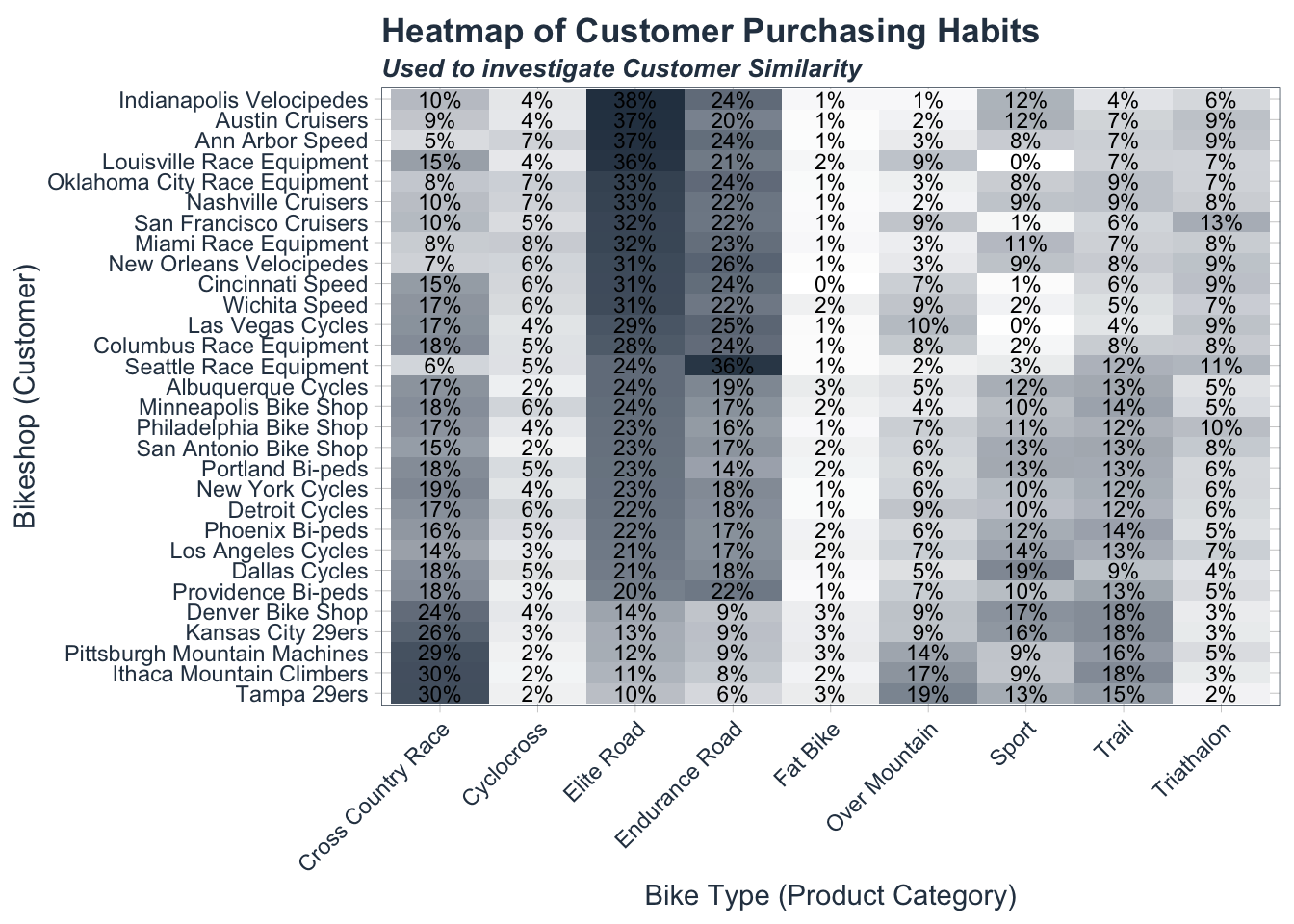
Heatmap

library(tidyverse)
library(tidyquant)

sales_by_customer_tbl <- read_rds("sales_by_customer.rds")
sales_by_customer_tbl

## # A tibble: 270 × 3
##    bikeshop_name      product_category   quantity
##    <fct>              <chr>                 <dbl>
##  1 Albuquerque Cycles Cross Country Race       48
##  2 Albuquerque Cycles Fat Bike                  9
##  3 Albuquerque Cycles Over Mountain            13
##  4 Albuquerque Cycles Sport                    35
##  5 Albuquerque Cycles Trail                    38
##  6 Albuquerque Cycles Cyclocross                7
##  7 Albuquerque Cycles Elite Road               69
##  8 Albuquerque Cycles Endurance Road           54
##  9 Albuquerque Cycles Triathalon               13
## 10 Ann Arbor Speed    Cross Country Race       32
## # … with 260 more rows

Data Wrangle

sales_by_customer_tbl %>% 
  group_by(bikeshop_name) %>% 
  mutate(prop = quantity / sum(quantity)) %>% 
  ungroup() %>% 
  select(- quantity) %>% 
  # AVOID THIS ROOKIE MISTAKE - DON'T FORGET TO SORT BY TOP PRODUCT ----
  pivot_wider(id_cols = bikeshop_name,
              names_from = product_category,
              values_from = prop) %>% 
  arrange(- `Elite Road`) %>% 
  mutate(bikeshop_name = fct_reorder(bikeshop_name, `Elite Road`)) %>% 
  pivot_longer(cols = - bikeshop_name,
               names_to = "product_category",
               values_to = "prop") -> prop_sales_by_customer_tbl
prop_sales_by_customer_tbl

## # A tibble: 270 × 3
##    bikeshop_name            product_category     prop
##    <fct>                    <chr>               <dbl>
##  1 Indianapolis Velocipedes Cross Country Race 0.103 
##  2 Indianapolis Velocipedes Fat Bike           0.0125
##  3 Indianapolis Velocipedes Over Mountain      0.0125
##  4 Indianapolis Velocipedes Sport              0.116 
##  5 Indianapolis Velocipedes Trail              0.0408
##  6 Indianapolis Velocipedes Cyclocross         0.0376
##  7 Indianapolis Velocipedes Elite Road         0.376 
##  8 Indianapolis Velocipedes Endurance Road     0.241 
##  9 Indianapolis Velocipedes Triathalon         0.0596
## 10 Austin Cruisers          Cross Country Race 0.0854
## # … with 260 more rows

Heatmap Visualization

prop_sales_by_customer_tbl %>% 
  ggplot(aes(product_category, bikeshop_name)) +
  # Geometirex
  geom_tile(aes(fill = prop)) + 
  geom_text(aes(label = scales::percent(prop, accuracy = 1)), size = 3) +
  # Formatting
  scale_fill_gradient(low = "white", high = palette_light()[1]) +
  labs(title = "Heatmap of Customer Purchasing Habits",
       subtitle = "Used to investigate Customer Similarity",
       x = "Bike Type (Product Category)",
       y = "Bikeshop (Customer)") +
  theme_tq() +
  theme(axis.text.x = element_text(angle = 45, hjust = 1),
        legend.position = "none",
        plot.title = element_text(face = "bold"),
        plot.subtitle = element_text(face = "bold.italic"))